Getting started with skore

This getting started guide illustrates how to use skore and why:

1. Track and visualize your ML/DS results using skore’s Project and UI.

2. Get assistance when developing your ML/DS projects.

   • Scikit-learn compatible skore.cross_validate() provides insights and checks on cross-validation.

Creating a skore project, loading it, and launching the UI

We start by creating a temporary directory to store our project such that we can easily clean it after executing this example. If you want to keep the project, you have to skip this section.

import tempfile
from pathlib import Path

temp_dir = tempfile.TemporaryDirectory(prefix="skore_example_")
temp_dir_path = Path(temp_dir.name)

From your shell, initialize a skore project, here named my_project:

import subprocess

# create the skore project
subprocess.run(
    f"python3 -m skore create my_project --working-dir {temp_dir.name}".split()
)

CompletedProcess(args=['python3', '-m', 'skore', 'create', 'my_project', '--working-dir', '/tmp/skore_example_ee6rrcxq'], returncode=0)

This will create a skore project directory named my_project.skore in your current directory.

From your shell (in the same directory), start the UI locally:

python -m skore launch "path/to/my_project"

This will automatically open a browser at the UI’s location.

Now that the project exists, we can write some Python code (in the same directory) to add (put()) some useful items in it. Let us load the project and add an integer to it for example:

from skore import load

my_project = load(temp_dir_path / "my_project.skore")
my_project.put("my_int", 3)

Example of machine learning usage: hyperparameter sweep

As an illustration of skore’s usage with a machine learning motivation, let us perform a hyperparameter sweep and store relevant information in the skore project.

We search for the alpha hyperparameter of a Ridge regression on the Diabetes dataset:

import numpy as np
from sklearn.datasets import load_diabetes
from sklearn.model_selection import GridSearchCV
from sklearn.linear_model import Ridge

diabetes = load_diabetes()
X = diabetes.data[:150]
y = diabetes.target[:150]

gs_cv = GridSearchCV(
    Ridge(),
    param_grid={"alpha": np.logspace(-3, 5, 50)},
    scoring="neg_root_mean_squared_error",
)
gs_cv.fit(X, y)

GridSearchCV(estimator=Ridge(),
             param_grid={'alpha': array([1.00000000e-03, 1.45634848e-03, 2.12095089e-03, 3.08884360e-03,
       4.49843267e-03, 6.55128557e-03, 9.54095476e-03, 1.38949549e-02,
       2.02358965e-02, 2.94705170e-02, 4.29193426e-02, 6.25055193e-02,
       9.10298178e-02, 1.32571137e-01, 1.93069773e-01, 2.81176870e-01,
       4.09491506e-01, 5.96362332e-01, 8.68511374e-01, 1.26485...
       3.72759372e+01, 5.42867544e+01, 7.90604321e+01, 1.15139540e+02,
       1.67683294e+02, 2.44205309e+02, 3.55648031e+02, 5.17947468e+02,
       7.54312006e+02, 1.09854114e+03, 1.59985872e+03, 2.32995181e+03,
       3.39322177e+03, 4.94171336e+03, 7.19685673e+03, 1.04811313e+04,
       1.52641797e+04, 2.22299648e+04, 3.23745754e+04, 4.71486636e+04,
       6.86648845e+04, 1.00000000e+05])},
             scoring='neg_root_mean_squared_error')

In a Jupyter environment, please rerun this cell to show the HTML representation or trust the notebook.
On GitHub, the HTML representation is unable to render, please try loading this page with nbviewer.org.

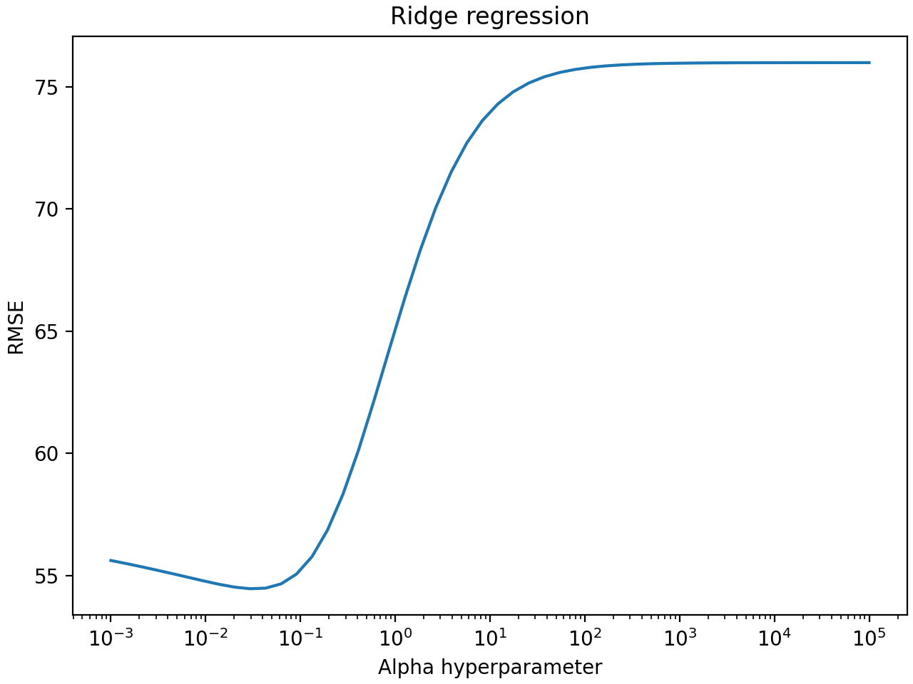
Now, we store the hyperparameter’s metrics in a dataframe and make a custom plot:

import pandas as pd

df = pd.DataFrame(gs_cv.cv_results_)
df.insert(len(df.columns), "rmse", -df["mean_test_score"].values)
df[["param_alpha", "rmse"]].head()

	param_alpha	rmse
0	0.001000	55.618873
1	0.001456	55.492536
2	0.002121	55.358884
3	0.003089	55.219924
4	0.004498	55.076585

import matplotlib.pyplot as plt

fig = plt.figure(layout="constrained", dpi=200)
plt.plot(df["param_alpha"], df["rmse"])
plt.xscale("log")
plt.xlabel("Alpha hyperparameter")
plt.ylabel("RMSE")
plt.title("Ridge regression")
plt.show()

Finally, we store some relevant information to our skore project, so that we can visualize them later in the skore UI for example:

my_project.put("my_gs_cv", gs_cv)
my_project.put("my_df", df)
my_project.put("my_fig", fig)

Cross-validation with skore

In order to assist its users when programming, skore has implemented a skore.cross_validate() function that wraps scikit-learn’s sklearn.model_selection.cross_validate(), to provide more context and facilitate the analysis.

For more information on the motivation behind skore’s cross_validate, see Enhancing cross-validation.

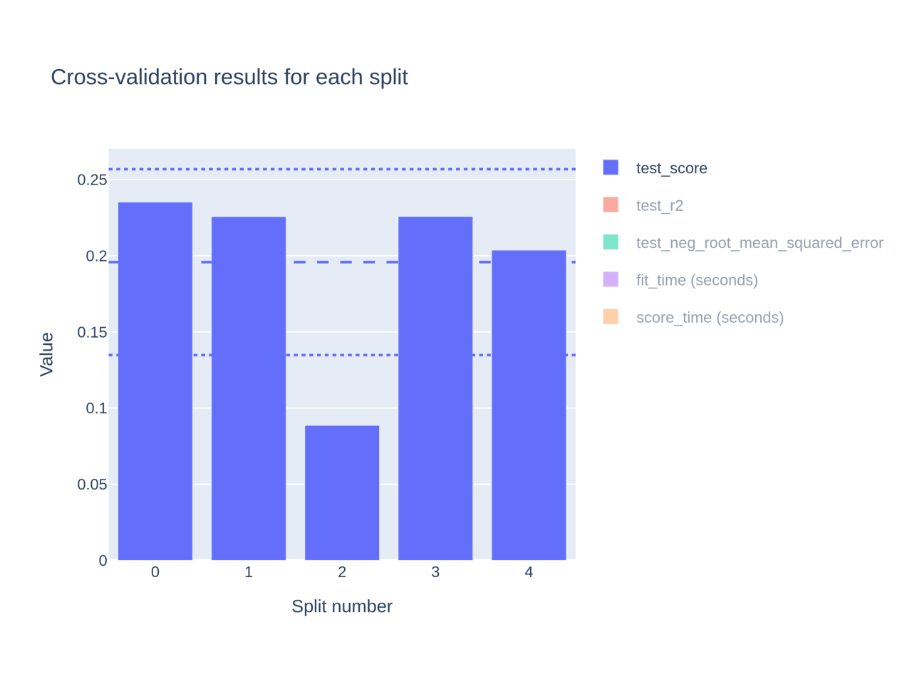
On the same previous data and a Ridge regressor (with default alpha value), let us launch skore’s cross-validation, which will automatically add (put()) a cross_validation item with a plotly chart in your project.

from skore import cross_validate

cv_results = cross_validate(Ridge(), X, y, cv=5, project=my_project)

fig_plotly = my_project.get_item("cross_validation").plot

Note

Because Plotly graphs currently do not properly render in our Sphinx auto-examples docs engine due to a bug in Plotly, we display its static image below.

import matplotlib.pyplot as plt
import matplotlib.image as mpimg

fig_plotly.write_image("plot_01_cross_validation.png", scale=4)

img = mpimg.imread("plot_01_cross_validation.png")
fig, ax = plt.subplots(layout="constrained", dpi=200)
ax.axis("off")
ax.imshow(img)
plt.show()

Manipulating the skore UI

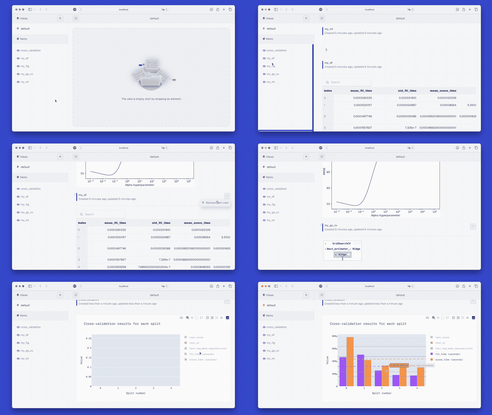
The skore UI is a very efficient tool to track and visualize the items in your project, such as grid search or cross-validation results.

1. On the top left, by default, you can observe that you are in a View called default. You can rename this view or create another one.

2. From the Items section on the bottom left, you can add stored items to this view, either by clicking on + or by doing drag-and-drop.

3. In the skore UI on the right, you can drag-and-drop items to re-order them, remove items, etc.

Cleanup the project

Remove the temporary directory:

temp_dir.cleanup()