Direct vs Recursive Forecasting

The purpose of this notebook is to compare the performance of direct forecasting and recursive forecasting using the MLForecast library. Direct forecasting means that we train a family of model to predict the target value at various horizons in the future, e.g. 1 hour, 2 hours, …, 24 hours ahead. Recursive forecasting (also known as auto-regressive forecasting) means that we train a single model to predict the target value at the next time step, and then use the model recursively to predict the next time step using the previous predictions as input features. Implementing recursive forecasting is a bit cumbersome to do manually, hence we use the MLForecast library to handle this for us.

The objective is to show that recursive forecasting can be more efficient in terms of memory usage and training time. However, it can also lead to a loss of accuracy because recursive calls are fed with previous predictions that do not necessarily match the training distribution of the model, and can therefore lead to degenerate predictions, in particular when the variance of the lagged values is informative.

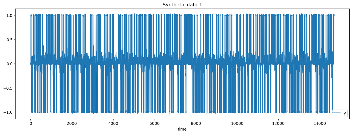
We highlight this issue with a synthetic dataset that has two types of segments:

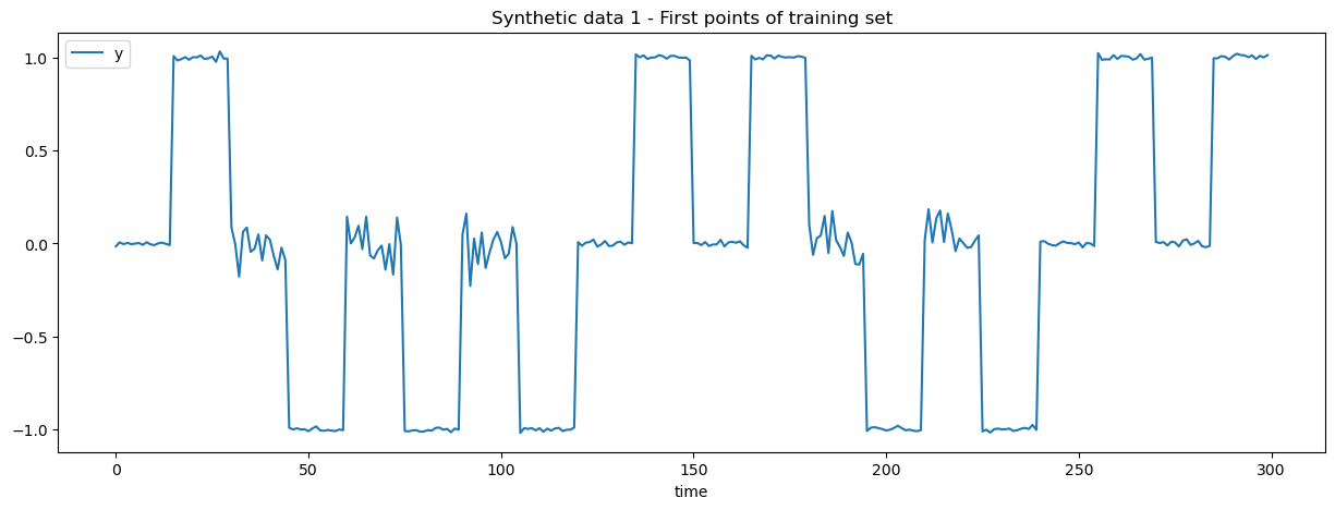
• Segment type “a” has a prefix centered around 0 with low variance and a suffix centered around 1 with low variance.

• Segment type “b” has a prefix centered around 0 with high variance and a suffix centered around -1 with low variance.

Segment of type “a” and “b” are independently sampled, meaning that is not possible to forecast beyond the length of the segments. However, it should be quite easy to predict the end of a segment given the prefix of the segment with lagged feature engineering.

from time import perf_counter
import numpy as np
import matplotlib.pyplot as plt
import pandas as pd
import tzdata  # noqa: F401

SEGMENT_LENGTH = 30


def generate_synthetic_1(
    segment_length=SEGMENT_LENGTH,
    n_segments=100,
    low_noise_level=0.01,
    high_noise_level=0.1,
    seed=None,
):
    """Generate synthetic time series data with two types of segments

    - segment type "a" has a prefix centered around 0 and a suffix centered
      around 1.
    - segment type "b" has a prefix centered around 0 with high variance and a
      suffix centered around -1.

    The variance of the prefix is therefore predictive of the suffix.

    The suffix values predictive of the next segment prefix's mean (always 0).
    """
    rng = np.random.default_rng(seed)
    total_length = segment_length * n_segments
    segment_types = rng.choice(["a", "b"], n_segments)
    prefix_length = segment_length // 2
    suffix_length = segment_length - prefix_length

    segments = []
    for segment_type in segment_types:
        if segment_type == "a":
            # Prefix is centered around 0 with low variance
            segments.append(
                rng.normal(loc=0, scale=low_noise_level, size=prefix_length)
            )
            # Suffix is centered around 1 with low variance
            segments.append(
                rng.normal(loc=1, scale=low_noise_level, size=suffix_length)
            )
        elif segment_type == "b":
            # Prefix is also centered around 0 but with high variance
            segments.append(
                rng.normal(loc=0, scale=high_noise_level, size=prefix_length)
            )
            # Suffix is centered around -1 with low variance
            segments.append(
                rng.normal(loc=-1, scale=low_noise_level, size=suffix_length)
            )
    return pd.DataFrame(
        {
            "time": np.arange(total_length),
            "y": np.concatenate(segments),
            "series_id": np.zeros(total_length, dtype=np.int32),
        }
    )


data = generate_synthetic_1(n_segments=500, seed=1)
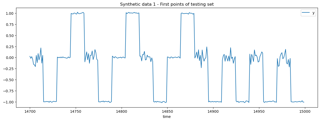
cutoff = -SEGMENT_LENGTH * 10  # 10 segments for testing
data_train = data.iloc[:cutoff]
data_test = data.iloc[cutoff:]
_ = data_train.plot(x="time", y="y", title="Synthetic data 1", figsize=(15, 5))

_ = data_train.iloc[: SEGMENT_LENGTH * 10].plot(
    x="time",
    y="y",
    title="Synthetic data 1 - First points of training set",
    figsize=(15, 5),
)

_ = data_test.iloc[: SEGMENT_LENGTH * 10].plot(
    x="time",
    y="y",
    title="Synthetic data 1 - First points of testing set",
    figsize=(15, 5),
)

from mlforecast import MLForecast
from sklearn.pipeline import make_pipeline
from sklearn.preprocessing import SplineTransformer, PolynomialFeatures
from sklearn.kernel_approximation import Nystroem
from mlforecast.lag_transforms import (
    RollingMax,
    RollingMin,
    RollingMean,
    RollingStd,
)
from mlforecast.target_transforms import Differences
from sklearn.linear_model import Ridge
from sklearn.ensemble import RandomForestRegressor, HistGradientBoostingRegressor
from sklearn.feature_selection import SelectKBest
from sklearn.tree import DecisionTreeRegressor
import warnings
import threadpoolctl

# Workaround a performance problem with HistGradientBoostingRegressor on small datasets.
threadpoolctl.threadpool_limits(limits=1, user_api="openmp")
warnings.filterwarnings("ignore", category=RuntimeWarning, module="sklearn")


# MLForecast can train multiple models in parallel, each model can be a
# pipeline of transformers and a regressor. However we focus on a single
# HistGradientBoostingRegressor model to make sure that this notebook runs
# quickly enough. Feel free to uncomment the other models to compare their
# performance if you have enough time and memory available.
#
# Spoiler alert: the HistGradientBoostingRegressor model is the most accurate.

mlf = MLForecast(
    models=[
        # make_pipeline(
        #     SplineTransformer(sparse_output=True, n_knots=10),
        #     PolynomialFeatures(degree=2, include_bias=False, interaction_only=True),
        #     # Nystroem(kernel="poly", n_components=200, degree=2, random_state=0),
        #     SelectKBest(k=100),
        #     Ridge(alpha=1e-6),
        # ),
        # RandomForestRegressor(
        #     n_estimators=100,
        #     max_features=0.8,
        #     max_depth=8,
        #     min_samples_leaf=300,
        #     n_jobs=4,
        # ),
        # DecisionTreeRegressor(max_depth=8, min_samples_leaf=300),
        HistGradientBoostingRegressor(),
    ],
    freq=1,
    lags=range(1, SEGMENT_LENGTH + 1),
    lag_transforms={
        1: [
            RollingMean(SEGMENT_LENGTH // 2),
            RollingStd(SEGMENT_LENGTH // 2),
        ],
        SEGMENT_LENGTH
        // 2: [
            RollingMax(SEGMENT_LENGTH // 2),
            RollingMin(SEGMENT_LENGTH // 2),
        ],
    },
    # target_transforms=[Differences([1])],
    num_threads=4,
)
schema = dict(
    time_col="time",
    id_col="series_id",
    target_col="y",
)

mlf.preprocess(data_train, **schema)

	time	y	series_id	lag1	lag2	lag3	lag4	lag5	lag6	lag7	...	lag25	lag26	lag27	lag28	lag29	lag30	rolling_mean_lag1_window_size15	rolling_std_lag1_window_size15	rolling_max_lag15_window_size15	rolling_min_lag15_window_size15
30	30	0.086113	0	0.992702	0.993013	1.031000	0.975424	1.003332	0.993741	0.990852	...	-0.000597	-0.003396	0.003249	-0.003548	0.006188	-0.015397	0.996924	0.013039	1.006198	-0.008697
31	31	-0.003983	0	0.086113	0.992702	0.993013	1.031000	0.975424	1.003332	0.993741	...	0.002458	-0.000597	-0.003396	0.003249	-0.003548	0.006188	0.935585	0.235347	1.006198	-0.008697
32	32	-0.177943	0	-0.003983	0.086113	0.992702	0.993013	1.031000	0.975424	1.003332	...	-0.007467	0.002458	-0.000597	-0.003396	0.003249	-0.003548	0.869826	0.337127	1.006198	-0.008697
33	33	0.062693	0	-0.177943	-0.003983	0.086113	0.992702	0.993013	1.031000	0.975424	...	0.006787	-0.007467	0.002458	-0.000597	-0.003396	0.003249	0.791984	0.429595	1.006198	-0.008697
34	34	0.085538	0	0.062693	-0.177943	-0.003983	0.086113	0.992702	0.993013	1.031000	...	-0.004699	0.006787	-0.007467	0.002458	-0.000597	-0.003396	0.729470	0.463953	1.006198	-0.008697
...	...	...	...	...	...	...	...	...	...	...	...	...	...	...	...	...	...	...	...	...	...
14695	14695	1.010180	0	1.000320	1.014936	1.003430	0.991600	0.998221	0.992632	0.989077	...	0.008091	0.999022	0.989610	1.017450	0.986895	1.000529	0.664467	0.489913	1.017450	-0.017102
14696	14696	1.019595	0	1.010180	1.000320	1.014936	1.003430	0.991600	0.998221	0.992632	...	0.010742	0.008091	0.999022	0.989610	1.017450	0.986895	0.731740	0.460728	1.017450	-0.017102
14697	14697	1.014361	0	1.019595	1.010180	1.000320	1.014936	1.003430	0.991600	0.998221	...	0.012473	0.010742	0.008091	0.999022	0.989610	1.017450	0.800022	0.417685	0.999022	-0.017102
14698	14698	0.987593	0	1.014361	1.019595	1.010180	1.000320	1.014936	1.003430	0.991600	...	-0.006401	0.012473	0.010742	0.008091	0.999022	0.989610	0.867881	0.355933	0.999022	-0.017102
14699	14699	1.002173	0	0.987593	1.014361	1.019595	1.010180	1.000320	1.014936	1.003430	...	-0.001378	-0.006401	0.012473	0.010742	0.008091	0.999022	0.934417	0.260507	0.012473	-0.017102

14670 rows × 37 columns

Recursive or auto-regressive forecasting

tic = perf_counter()
mlf.fit(data_train, **schema)  # recursive forecasting by default in mlforecast
print(f"Recursive forecasting training time: {perf_counter() - tic:.1f} seconds")

Recursive forecasting training time: 0.4 seconds

PREDICTION_HORIZON = SEGMENT_LENGTH * 2


def collect_predictions(mlf, data_test, test_offset=0):
    """Collect predictions from the MLForecast object."""
    all_predictions = []
    UPDATE_CHUNK_SIZE = 5
    while test_offset < len(data_test):

        new_predictions = mlf.predict(PREDICTION_HORIZON)
        new_predictions["horizon"] = np.arange(new_predictions.shape[0]) + 1
        new_predictions = new_predictions.merge(
            data_test, on=["time", "series_id"], how="left"
        )
        all_predictions.append(new_predictions)

        # Update the forecaster with the new observations
        mlf.update(data_test.iloc[test_offset : test_offset + UPDATE_CHUNK_SIZE])
        test_offset += UPDATE_CHUNK_SIZE

    return all_predictions


tic = perf_counter()
all_recursive_predictions = collect_predictions(mlf, data_test)
print(f"Recursive forecasting prediction time: {perf_counter() - tic:.1f} seconds")

Recursive forecasting prediction time: 27.8 seconds

Direct forecasting

Let’s pass max_horizon to force modeling for direct forecasting.

tic = perf_counter()
mlf.fit(data_train, max_horizon=PREDICTION_HORIZON, **schema)
print(f"Direct forecasting training time: {perf_counter() - tic:.1f} seconds")

Direct forecasting training time: 17.6 seconds

tic = perf_counter()
all_direct_predictions = collect_predictions(mlf, data_test)
print(f"Direct forecasting prediction time: {perf_counter() - tic:.1f} seconds")

Direct forecasting prediction time: 4.5 seconds

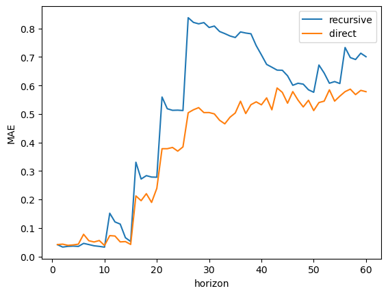
Quantitative comparison

def score_predictions(all_predictions, model_name):
    """Compute the mean absolute error of the predictions."""
    all_predictions = pd.concat(all_predictions)
    all_predictions["absolute_error"] = np.abs(
        all_predictions["y"] - all_predictions[model_name]
    )
    return all_predictions.dropna().groupby("horizon")


import matplotlib.pyplot as plt

fig, ax = plt.subplots()
score_predictions(
    all_recursive_predictions, "HistGradientBoostingRegressor"
).mean().reset_index().plot(x="horizon", y="absolute_error", label="recursive", ax=ax)
score_predictions(
    all_direct_predictions, "HistGradientBoostingRegressor"
).mean().reset_index().plot(x="horizon", y="absolute_error", label="direct ", ax=ax)
_ = ax.set(ylabel="MAE")

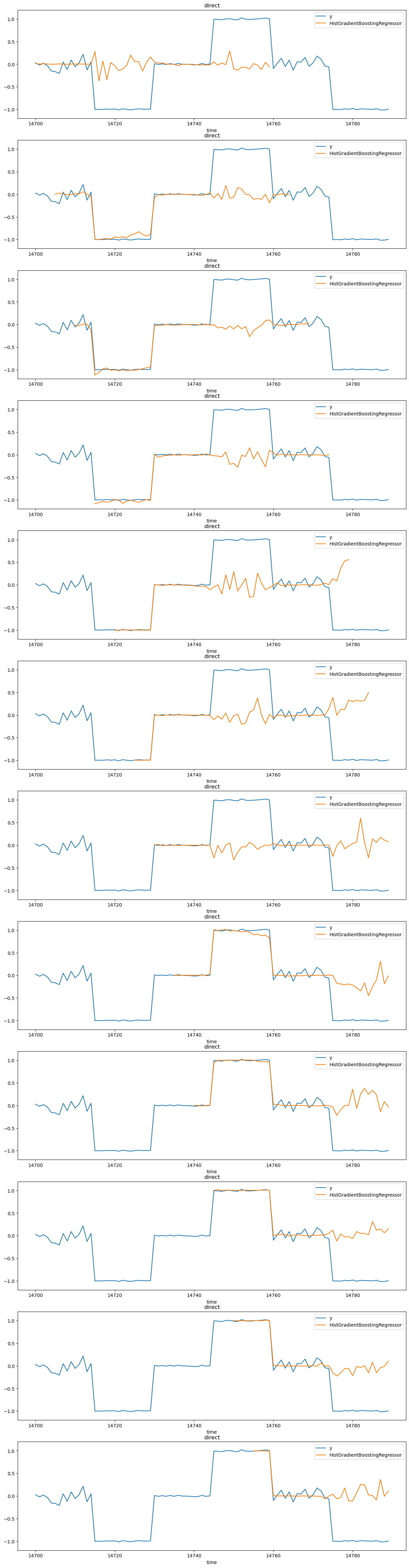
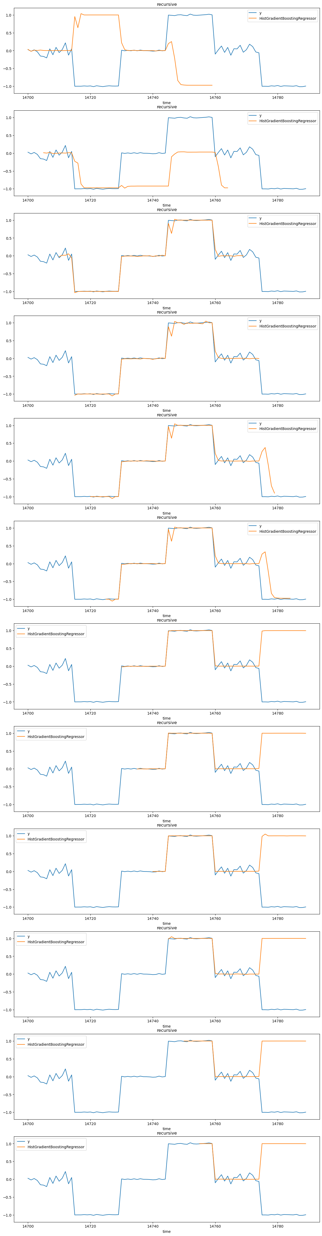
Qualitative comparison

def plot_some_predictions(all_predictions, data_test, model_name, nrows=12, title=None):

    fig, axes = plt.subplots(nrows=nrows, figsize=(15, 5 * nrows))
    for row_idx, predictions in enumerate(all_predictions):
        predictions = predictions.drop("y", axis=1)
        merged_data = data_test.copy()
        merged_data = merged_data.merge(
            predictions, on=["time", "series_id"], how="left"
        )
        merged_data.drop(["series_id"], axis=1).iloc[: SEGMENT_LENGTH * 3].plot(
            x="time", y=["y", model_name], ax=axes[row_idx]
        )
        axes[row_idx].set_title(title)
        axes[row_idx].set_ylim(-1.2, 1.2)

        if row_idx >= nrows - 1:
            break

plot_some_predictions(
    all_recursive_predictions,
    data_test,
    "HistGradientBoostingRegressor",
    title="recursive",
)

plot_some_predictions(
    all_direct_predictions, data_test, "HistGradientBoostingRegressor", title="direct"
)