Cost-sensitive learning to optimize business metrics#
Many real-world applications of machine learning aim to automate operational decisions with access to partial contextual information. This requires designing a decision policy that is optimal with respect to some given “utility function” or “business metric”. The aim is therefore to maximize a gain or minimize a cost that is related to the decision taken by the system (for instance accept or reject a transaction) prior to the observation of a delayed outcome (discovering that the transaction was legitimate or fraudulent) modeled as a target random variable conditioned on observed contextual information.
In this tutorial, we explore the concrete example of fraud detection in credit card transactions. We first describe the dataset used to train our predictive models and the function used to evaluate the resulting operational decisions. Then, we design a few machine learning based decision system of increasing sophistication and compare their business performance to baselines and oracle decisions on held out data.
The credit card dataset#
The dataset is available on OpenML at the following URL.
We have a local copy of the dataset in the datasets folder. Let’s load the
parquet file and check the data that we have at hand.
import pandas as pd

# `pandas` automatically selects a parquet engine: `pyarrow` is bundled with
# Pyodide for the in-browser JupyterLite build, while `fastparquet` is used in
# the local/CI environment.
credit_card = pd.read_parquet("../datasets/credit_card.parquet")
credit_card.info()
<class 'pandas.core.frame.DataFrame'>
RangeIndex: 284807 entries, 0 to 284806
Data columns (total 31 columns):
 #   Column  Non-Null Count   Dtype
---  ------  --------------   -----
 0   Time    284807 non-null  float64
 1   V1      284807 non-null  float64
 2   V2      284807 non-null  float64
 3   V3      284807 non-null  float64
 4   V4      284807 non-null  float64
 5   V5      284807 non-null  float64
 6   V6      284807 non-null  float64
 7   V7      284807 non-null  float64
 8   V8      284807 non-null  float64
 9   V9      284807 non-null  float64
 10  V10     284807 non-null  float64
 11  V11     284807 non-null  float64
 12  V12     284807 non-null  float64
 13  V13     284807 non-null  float64
 14  V14     284807 non-null  float64
 15  V15     284807 non-null  float64
 16  V16     284807 non-null  float64
 17  V17     284807 non-null  float64
 18  V18     284807 non-null  float64
 19  V19     284807 non-null  float64
 20  V20     284807 non-null  float64
 21  V21     284807 non-null  float64
 22  V22     284807 non-null  float64
 23  V23     284807 non-null  float64
 24  V24     284807 non-null  float64
 25  V25     284807 non-null  float64
 26  V26     284807 non-null  float64
 27  V27     284807 non-null  float64
 28  V28     284807 non-null  float64
 29  Amount  284807 non-null  float64
 30  Class   284807 non-null  category
dtypes: category(1), float64(30)
memory usage: 65.5 MB
The target column is the “Class” column. It informs us whether a transaction is fraudulent (class 1) or legitimate (class 0).
We see a set of features that are anonymized starting with “V”. Looking at the dataset description in OpenML, we learn that those features are the result of a PCA transformation. The only non-transformed features are the “Time” and “Amount” columns. The “Time” corresponds to the number of seconds elapsed between this transaction and the first transaction in the dataset. The “Amount” is the amount of the transaction.
We first extract the target column from the other columns used as inputs to our predictive model:
target_name = "Class"
data = credit_card.drop(columns=[target_name, "Time"])
target = credit_card[target_name].astype(int)
The credit card fraud detection problem also has a special characteristic: the dataset is highly imbalanced. We can check the distribution of the target to confirm this.
target.value_counts(normalize=True)
Class
0    0.998273
1    0.001727
Name: proportion, dtype: float64
The dataset is highly imbalanced with fraudulent transactions representing only 0.17% of the data. Since we are interested in training a machine learning model, we should also make sure that we have enough data points in the minority class to train the model by looking at the absolute numbers of transactions of each class.
target.value_counts()
Class
0    284315
1       492
Name: count, dtype: int64
We observe that we have around 500 data points for the minority class. This is on the low end of the number of data points required to train a machine learning model successfully.
In addition of the target distribution, we check the distribution of the amount of the legitimate and fraudulent separately transactions.
import numpy as np
import matplotlib.pyplot as plt

amount_groupby_class = pd.concat([data["Amount"], target], axis=1).groupby("Class")[
    "Amount"
]

_, ax = plt.subplots(ncols=2, figsize=(12, 6), sharex=True, sharey=True)
bins = np.linspace(0, data["Amount"].max(), 30)
for class_id, amount in amount_groupby_class:
    ax[class_id].hist(amount, bins=bins, edgecolor="black", density=True)
    ax[class_id].set(
        xlabel="Amount (€)",
        ylabel="Ratio of transactions",
        xscale="log",
        yscale="log",
        title=(
            "Distribution of the amount of "
            f'{"fraudulent" if class_id else "legitimate"} transactions'
        ),
    )
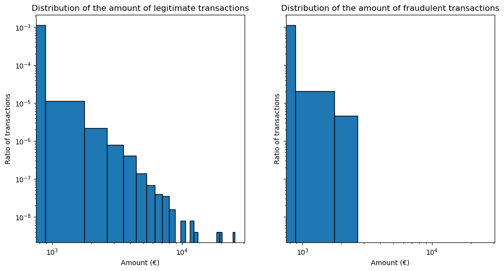
We cannot conclude a particular pattern in the distribution of the amount of the transactions apart from the fact that none of the fraudulent transactions has a very large amount. This information could be useful: if we train a predictive model on these data, we should consider that we do not know how our predictive model will behave on fraudulent transactions with large amounts in the future. It might be worth considering to have a specific treatment for those transactions.
Evaluating decisions with a business metric#
Now, we create the business metric that depends on the amount of each transaction.
The gain of a legitimate transaction is quite easy to define since it is a commission that the operator receives. Here, we define it to be 2% of the amount of the transaction. Similarly, there is no gain in refusing a fraudulent transaction: the operator does not receive money from external actors or clients in this case.
Defining a cost for refusing a legitimate transaction or accepting a fraudulent transaction is more complex. If the operator accepts a fraudulent transaction, it loses the amount of the transaction. There is also an extra cost involved that we define as the sum of several other costs: the cost of the fraud investigation, the cost of the customer support, and the cost related to brand reputation damage. Those additional costs should be specified by the data scientist in collaboration with the business stakeholders. A similar approach should be taken for the cost of refusing a legitimate transaction: the cost of customer support and the cost of a customer churning multiplied by estimated contribution of rejecting a legitimate transaction on churning.
# Commission received for each accepted legitimate transaction
commission_transaction_gain = 0.02
# Expected extra cost of accepting a fraudulent transaction
avg_accept_fraud_cost = 20
# Expected cost of refusing a legitimate transaction
avg_refuse_legit_cost = 10


def business_gain_func(y_true, y_pred, amount):
    """Business metric to optimize.

    The terms computed in this function are expressed in terms of gain. It means that
    the diagonal entry of the gain matrix G_00 and G_11 are positive values and the
    other entries are negative values. The off-diagonal entries are however negative
    values (a cost is considered as a negative gain).
    """
    true_negative_g00 = (y_pred == 0) & (y_true == 0)
    false_negative_g01 = (y_pred == 0) & (y_true == 1)
    false_positive_g10 = (y_pred == 1) & (y_true == 0)
    true_positive_g11 = (y_pred == 1) & (y_true == 1)

    accept_legitimate = (amount[true_negative_g00] * commission_transaction_gain).sum()
    accept_fraudulent = -(
        amount[false_negative_g01].sum()
        + (false_negative_g01 * avg_accept_fraud_cost).sum()
    )
    refuse_legitimate = -(false_positive_g10 * avg_refuse_legit_cost).sum()
    refuse_fraudulent = (true_positive_g11 * 0).sum()

    return accept_legitimate + accept_fraudulent + refuse_legitimate + refuse_fraudulent
We further wrap this metric function as a scikit-learn scorer object that computes the business metric given a fitted classifier and a test set. This scorer is handy because it can be used in meta-estimators, grid-search, and cross-validation.
To create this scorer, we use the sklearn.metrics.make_scorer factory. The
metric defined above requests the amount of each transaction. This variable
is an additional metadata to be passed to the scorer and we need to use
scikit-learn’s metadata routing mechanism to pass this side information where
appropriate.
import sklearn
from sklearn.metrics import make_scorer

sklearn.set_config(enable_metadata_routing=True)
business_gain_scorer = make_scorer(business_gain_func).set_score_request(amount=True)
So at this stage, we see that the amount of the transaction is used twice: once as a
feature to train our predictive model and once as a metadata to compute the the
business metric and thus the business performance of our model. When used as a
feature, we are only required to have a column in data that contains the amount of
each transaction. To use this information as metadata, we need to have an external
variable that we can pass to the scorer or the model that internally routes
this metadata to the scorer. So let’s extract this variable as a standalone
numpy array:
amount = credit_card["Amount"].to_numpy()
Investigate baseline policies#
Before to train a machine learning model, we investigate some baseline policies to serve as reference. Also, we prepare our dataset, to have a left-out test set to evaluate the performance of our predictive model.
from sklearn.model_selection import train_test_split

data_train, data_test, target_train, target_test, amount_train, amount_test = (
    train_test_split(
        data, target, amount, stratify=target, test_size=0.5, random_state=42
    )
)
The first baseline policy to evaluate is to check the performance of a policy that always accepts the transaction. We recall that class “0” is the legitimate class and class “1” is the fraudulent class.
from sklearn.dummy import DummyClassifier

always_accept_policy = DummyClassifier(strategy="constant", constant=0)
always_accept_policy.fit(data_train, target_train)
benefit = business_gain_scorer(
    always_accept_policy, data_test, target_test, amount=amount_test
)
print(f"Benefit of the 'always accept' policy: {benefit:,.2f}€")
Benefit of the 'always accept' policy: 216,525.07€
A decision policy that considers all transactions as legitimate and as result never rejects a transaction would yield a total profit around 216,000€.
We further evaluate a policy that rejects all transactions as fraudulent:
always_reject_policy = DummyClassifier(strategy="constant", constant=1)
always_reject_policy.fit(data_train, target_train)
benefit = business_gain_scorer(
    always_reject_policy, data_test, target_test, amount=amount_test
)
print(f"Benefit of the 'always reject' policy: {benefit:,.2f}€")
Benefit of the 'always reject' policy: -1,421,580.00€
Such a policy would entail a catastrophic loss: around 1,421,000€. This is expected since the vast majority of the transactions are legitimate and the policy would refuse them at a non-trivial cost and never collect any commission.
Now, we evaluate a hypothetical oracle policy that would know exactly which transactions are fraudulent before making the decision to accept or reject:
business_score = business_gain_func(
    target_test,
    target_test,
    amount=amount_test,
)
print(f"Benefit of oracle decisions (not reachable):  {business_score:,.2f}€")
Benefit of oracle decisions (not reachable): 251,031.83€
This perfect model would make a profit of around 251,000€.
Therefore, we conclude that a predictive model that a model which adapts the accept/reject decisions on a per transaction basis should ideally allow us to make a profit larger than the ~216,000€ and will be capped by an amount of ~251,000€ of the best of our constant baseline policies.
Training predictive models#
Logistic regression tuned with a proper scoring rule#
We start by training a logistic regression model with the default decision
threshold at 0.5. Here we tune the hyperparameter C of the logistic
regression with a proper scoring rule (the log loss) to ensure that the
model’s probabilistic predictions returned by its predict_proba method are
as accurate as possible, irrespectively of the choice of the value of the
decision threshold.
from sklearn.linear_model import LogisticRegression
from sklearn.model_selection import GridSearchCV
from sklearn.pipeline import make_pipeline
from sklearn.preprocessing import StandardScaler

logistic_regression = make_pipeline(StandardScaler(), LogisticRegression())
param_grid = {"logisticregression__C": np.logspace(-6, 6, 13)}
model = GridSearchCV(logistic_regression, param_grid, scoring="neg_log_loss")
model.fit(data_train, target_train)
GridSearchCV(estimator=Pipeline(steps=[('standardscaler', StandardScaler()),
                                       ('logisticregression',
                                        LogisticRegression())]),
             param_grid={'logisticregression__C': array([1.e-06, 1.e-05, 1.e-04, 1.e-03, 1.e-02, 1.e-01, 1.e+00, 1.e+01,
       1.e+02, 1.e+03, 1.e+04, 1.e+05, 1.e+06])},
             scoring='neg_log_loss')
In a Jupyter environment, please rerun this cell to show the HTML representation or trust the notebook. On GitHub, the HTML representation is unable to render, please try loading this page with nbviewer.org.
Parameters
Fitted attributes
Parameters
Fitted attributes
29 features
| V1 |
| V2 |
| V3 |
| V4 |
| V5 |
| V6 |
| V7 |
| V8 |
| V9 |
| V10 |
| V11 |
| V12 |
| V13 |
| V14 |
| V15 |
| V16 |
| V17 |
| V18 |
| V19 |
| V20 |
| V21 |
| V22 |
| V23 |
| V24 |
| V25 |
| V26 |
| V27 |
| V28 |
| Amount |
Parameters
Fitted attributes
model.best_params_
{'logisticregression__C': np.float64(100.0)}
print(
    "Benefit of logistic regression with default threshold: "
    f"{business_gain_scorer(model, data_test, target_test, amount=amount_test):,.2f}€"
)
Benefit of logistic regression with default threshold: 235,234.87€
The business metric shows that our predictive model with a default decision threshold is already winning over the baseline in terms of profit and it would be already beneficial to use it to accept or reject transactions instead of accepting all transactions.
However there is no reason to believe that this particular choice of decision threshold would be optimal for the problem at hand.
Setting the decision threshold by direct business metric optimization#
In the previous section, we presented a method to compute the optimal decision threshold but it relied on the assumption that the probabilistic classifier is well-calibrated and that the business metric can be expressed as a cost matrix.
Furthermore, the threshold computed with the closed form formula depends on the amount of the transaction. Since we wanted to used a fixed threshold for all decisions, we naively used the mean optimal threshold. This further breaks any optimality guarantee.
To avoid relying on such assumptions, we can instead tune a single decision
threshold by directly optimizing the average business metric. This
optimization is done through a grid-search over the decision threshold
involving a cross-validation. The class
sklearn.model_selection.TunedThresholdClassifierCV is in charge of
performing this optimization.
from sklearn.model_selection import TunedThresholdClassifierCV

tuned_model = TunedThresholdClassifierCV(
    estimator=model.best_estimator_,
    scoring=business_gain_scorer,
    thresholds=100,
    n_jobs=2,
    store_cv_results=True,
)
tuned_model
TunedThresholdClassifierCV(estimator=Pipeline(steps=[('standardscaler',
                                                      StandardScaler()),
                                                     ('logisticregression',
                                                      LogisticRegression(C=np.float64(100.0)))]),
                           n_jobs=2,
                           scoring=make_scorer(business_gain_func, response_method='predict'),
                           store_cv_results=True)
In a Jupyter environment, please rerun this cell to show the HTML representation or trust the notebook. On GitHub, the HTML representation is unable to render, please try loading this page with nbviewer.org.
Parameters
Parameters
Parameters
Parameters
Since our business scorer requires the amount of each transaction, we need to
pass this information in the fit method. The
sklearn.model_selection.TunedThresholdClassifierCV is in charge of
automatically dispatching this metadata to the underlying scorer.
tuned_model.fit(data_train, target_train, amount=amount_train)
TunedThresholdClassifierCV(estimator=Pipeline(steps=[('standardscaler',
                                                      StandardScaler()),
                                                     ('logisticregression',
                                                      LogisticRegression(C=np.float64(100.0)))]),
                           n_jobs=2,
                           scoring=make_scorer(business_gain_func, response_method='predict'),
                           store_cv_results=True)
In a Jupyter environment, please rerun this cell to show the HTML representation or trust the notebook. On GitHub, the HTML representation is unable to render, please try loading this page with nbviewer.org.
Parameters
Fitted attributes
Parameters
Fitted attributes
Parameters
Fitted attributes
29 features
| V1 |
| V2 |
| V3 |
| V4 |
| V5 |
| V6 |
| V7 |
| V8 |
| V9 |
| V10 |
| V11 |
| V12 |
| V13 |
| V14 |
| V15 |
| V16 |
| V17 |
| V18 |
| V19 |
| V20 |
| V21 |
| V22 |
| V23 |
| V24 |
| V25 |
| V26 |
| V27 |
| V28 |
| Amount |
Parameters
Fitted attributes
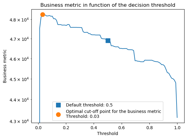
Let’s compare the decision threshold found by the model compared to our fixed global threshold from the previous section.
tuned_model.best_threshold_
np.float64(0.03030303030292765)
The resulting threshold value is much lower than the default of 0.5.
Now, let’s check the performance of our model with the tuned decision threshold by computing the value of the business metric on the test set:
print(
    "Benefit of logistic regression with a tuned threshold: "
    f"{business_gain_scorer(tuned_model, data_test, target_test, amount=amount_test):,.2f}€"
)
Benefit of logistic regression with a tuned threshold: 238,123.39€
We see that adjusting the decision threshold increases the gains compared to using the default 0.5 threshold of scikit-learn classifiers.
Let’s have a look at the relationship between the decision threshold and the
business metric by inspecting the fitted attributes of the
TunedThresholdClassifierCV instance:
_, ax = plt.subplots()
ax.semilogy(
    tuned_model.cv_results_["thresholds"],
    tuned_model.cv_results_["scores"],
    color="tab:blue",
)

# Replace vertical line with a single point for default threshold
default_score = tuned_model.cv_results_["scores"][
    np.abs(tuned_model.cv_results_["thresholds"] - 0.5).argmin()
]
ax.semilogy(
    0.5,
    default_score,
    "s",  # square marker
    markersize=10,
    color="tab:blue",
    label="Default threshold: 0.5",
)

ax.semilogy(
    tuned_model.best_threshold_,
    tuned_model.best_score_,
    "o",
    markersize=10,
    color="tab:orange",
    label=(
        f"Optimal cut-off point for the business metric\n"
        f"Threshold: {tuned_model.best_threshold_:.2f}"
    ),
)
ax.set(
    xlabel="Threshold",
    ylabel="Business metric",
    title="Business metric in function of the decision threshold",
)
_ = ax.legend()
Tuned logistic regression with optimal decision threshold#
From a research paper by Charles Elkan [1], we know that the optimal decision threshold for a problem with a binary outcome can be computed by a closed-form formula given the following two assumptions:
the probabilistic classifier is well-calibrated,
the business metric can be decomposed as the sum of entries of a cost (or gain) matrix.
When defining our business metric, we have already expressed it as a gain matrix. So to use the approach described in [1], we only need to check the calibration of our model. In the previous section, we already tuned the hyperparameter of the logistic regression using a proper scoring rule that should help towards getting a well-calibrated model. As a first step, we assume that our classifier is well-calibrated. Later, we will add an extra calibration step to check if it improves the performance of our model in terms of the business metric.
The optimal decision threshold proposed by Charles Elkan in [1] is defined as follows:
def elkan_optimal_threshold(amount):
    """Compute the optimal threshold for a transaction of a given amount.

    Here the terms are expressed as costs. Therefore, the diagonal entries of the
    cost matrix (C_00 and C_11) are negative values and the off-diagonal values
    are positive.

    Note that we can multiply the numerator and the denominator by -1 to yield
    the same formula for the entries of a gain matrix. The resulting threshold
    would stay unchanged.
    """
    c00 = -commission_transaction_gain * amount  # Accepting a legitimate transaction
    c01 = amount + avg_accept_fraud_cost  # Accepting a fraudulent transaction
    c10 = avg_refuse_legit_cost  # Refusing a legitimate transaction
    c11 = 0  # Refusing a fraudulent transaction
    return (c10 - c00) / (c10 - c00 + c01 - c11)
Let’s plot the distribution of the optimal thresholds for the transactions in the train set. In addition, we plot the optimal threshold as a function of the transaction amount.
_, ax = plt.subplots(ncols=2, figsize=(14, 6))

ax[0].hist(elkan_optimal_threshold(amount_train), bins=100, edgecolor="black")
ax[0].set(
    xlabel="Optimal threshold",
    ylabel="Number of transactions",
    title="Optimal threshold distribution",
)

x = np.linspace(amount_train.min(), amount_train.max(), 1_000)
ax[1].plot(x, elkan_optimal_threshold(x))
_ = ax[1].set(
    xlabel="Amount (€)",
    ylabel="Optimal threshold",
    title="Optimal threshold in function of the transaction amount",
)
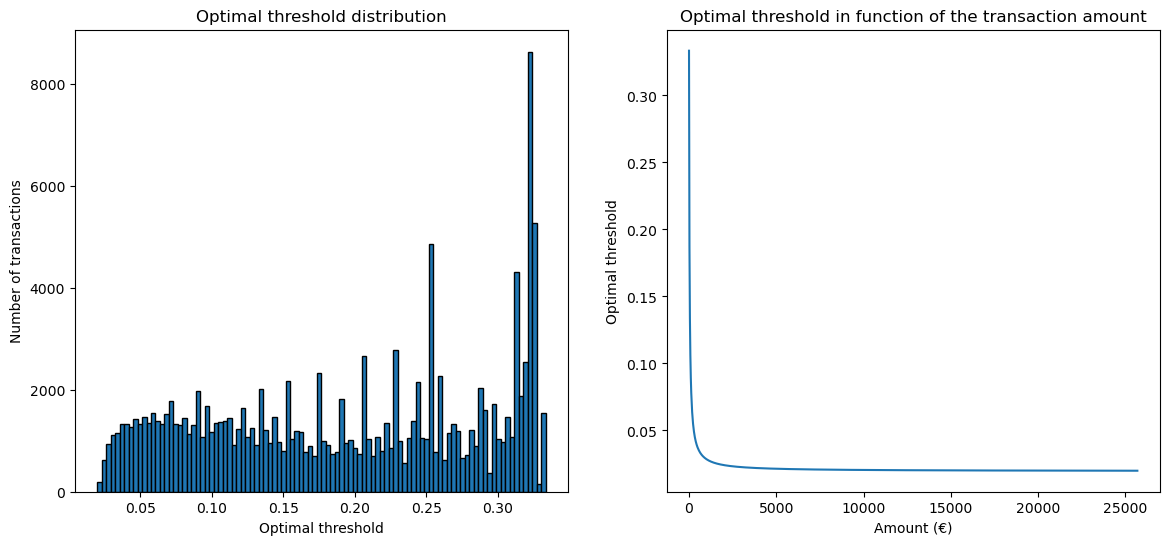
We see that the optimal threshold varies from ~0.02 to ~0.33 depending on the amount of the transaction. Looking at the optimal threshold as a function of the transaction amount, we see that it decreases as the amount of the transaction increases. It means that the operator should reject a transaction with a large amount unless it is extremely confident that this a legitimate transaction. For lower amounts, it is optimal to take more risk and accept transactions with higher estimated probability of being fraudulent.
As a first experiment, we define a decision policy with a constant decision threshold computed as the mean of the optimal thresholds computed for the transactions in the train set. Let’s check the value of this threshold:
elkan_optimal_threshold(amount_train).mean()
np.float64(0.19305440698357446)
Let’s use this value to change the decision threshold of our logistic regression model and evaluate the performance of our model in terms of the business metric.
from sklearn.model_selection import FixedThresholdClassifier

fixed_elkan_model = FixedThresholdClassifier(
    estimator=model.best_estimator_,
    threshold=elkan_optimal_threshold(amount_train).mean(),
).fit(data_train, target_train)

business_score = business_gain_scorer(
    fixed_elkan_model, data_test, target_test, amount=amount_test
)

print(
    f"Benefit of logistic regression with a fixed mean theoretical threshold: "
    f"{business_score:,.2f}€"
)
Benefit of logistic regression with a fixed mean theoretical threshold: 236,756.32€
We see that adjusting the decision threshold increases the gains compared to
using the default 0.5 threshold of scikit-learn classifiers but not as good
as the threshold found via TunedThresholdClassifierCV.
Note that the formula we used to compute the threshold is only valid under the following assumptions:
our model is well-calibrated,
our decisions are thresholded with amount dependent thresholds instead of using the mean optimal threshold.
Let’s first focus on calibration. Since the dataset is very imbalanced, our classifiers predicts very low probability for the fraudulent class most of the time, as a result use plot the calibration curve with a logarithmic scale:
from sklearn.calibration import CalibrationDisplay

disp = CalibrationDisplay.from_estimator(
    model.best_estimator_,
    data_test,
    target_test,
    strategy="quantile",
    n_bins=3,
    name="Tuned logistic regression",
)
_ = disp.ax_.set(xlim=(1e-7, 0.03), ylim=(1e-7, 0.03), xscale="log", yscale="log")
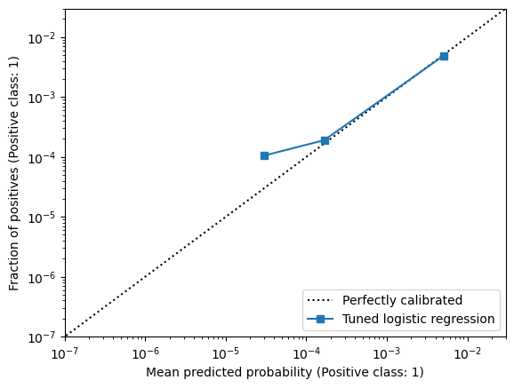
The calibration looks good but not perfect (not exactly on the diagonal). We use a small number of bins because there are very few fraudulent cases in the test data (less than 100 fraud cases per bin).:
target_test.value_counts()
Class
0    142158
1       246
Name: count, dtype: int64
If we had a larger dataset, we could use more bins to get a finer grained estimate of the calibration curve.
Despite this lack of data, let’s attempt to improve the calibration of our
classifier. Since we have little fraudulent data, we cannot afford to use a
held out calibration set. Instead we use a nested cross-fitting procedure
implemented in CalibratedClassifierCV: our original training set is
splitted 10 times into train and calibration subsets and we train 10
classifiers paired with 10 isotonic calibrators, one pair for each split:
from sklearn.calibration import CalibratedClassifierCV
from sklearn.model_selection import ShuffleSplit

calibrated_estimator = CalibratedClassifierCV(
    model.best_estimator_,
    method="isotonic",
    cv=ShuffleSplit(n_splits=10, test_size=0.2, random_state=42),
).fit(data_train, target_train)
disp = CalibrationDisplay.from_estimator(
    calibrated_estimator, data_test, target_test, strategy="quantile", n_bins=3
)
_ = disp.ax_.set(xlim=(1e-7, 0.03), ylim=(1e-7, 0.03), xscale="log", yscale="log")
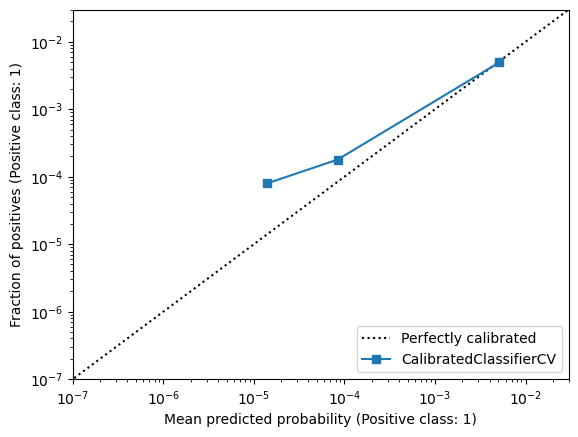
The calibration curve of the resulting model does not look significantly better than that of the original logistic regression model.
Still, let’s see of the cross-fitted calibration procedure can lead to an improvement measured with the business metric:
fixed_elkan_model = FixedThresholdClassifier(
    estimator=calibrated_estimator,
    threshold=elkan_optimal_threshold(amount_train).mean(),
).fit(data_train, target_train)

business_score = business_gain_scorer(
    fixed_elkan_model, data_test, target_test, amount=amount_test
)

print(
    f"Benefit of recalibrated logistic regression with a fixed mean theoretical "
    f" threshold:  {business_score:,.2f}€"
)
Benefit of recalibrated logistic regression with a fixed mean theoretical threshold: 238,327.63€
It seems that this extra calibration step did improve the performance of our
model in terms of the business metric. We are now very close to the business
metric value obtained with the fixed threshold found by
TunedThresholdClassifierCV on the uncalibrated model.
However, since we have very few fraudulent cases, this result should be confirmed on a larger dataset with more cases. Alternatively the robustness of this improvement should be assessed via an outer cross-validation instead of using a single global train test split.
Let’s now explore if using a per-transaction variable threshold can further improve this result.
Variable optimal threshold#
As we previously mentioned, the optimal threshold depends on each the amount
of each transaction. However FixedThresholdClassifier does not support
using variable thresholds.
So instead let’s write our own wrapper class to implement amount-dependent
thresholds in the predict method:
class VariableThresholdClassifier:

    def __init__(self, classifier, variable_threshold):
        self.classifier = classifier
        self.variable_threshold = variable_threshold

    def fit(self, X, y):
        return self

    def predict(self, X, amount):
        proba = self.classifier.predict_proba(X)[:, 1]
        return (proba >= self.variable_threshold(amount)).astype(np.int32)
This meta-estimator wraps a trained probabilistic classifier and computes the optimal threshold for each of the predictions and compare it with the classifier’s probability predictions. We now evaluate the performance of this model on the test set.
business_score = business_gain_func(
    target_test,
    VariableThresholdClassifier(
        model.best_estimator_,
        variable_threshold=elkan_optimal_threshold,
    ).predict(data_test, amount=amount_test),
    amount=amount_test,
)
print(
    f"Benefit of logistic regression with optimal variable threshold: "
    f"{business_score:,.2f}€"
)
Benefit of logistic regression with optimal variable threshold: 237,032.00€
We see that the profit is almost the same as the one obtained with the previous models Let’s now try to combine variable thresholding with post-hoc calibration of the underlying classifier:
business_score = business_gain_func(
    target_test,
    VariableThresholdClassifier(
        calibrated_estimator,
        variable_threshold=elkan_optimal_threshold,
    ).predict(data_test, amount=amount_test),
    amount=amount_test,
)
print(
    f"Benefit of recalibrated logistic regression with optimal variable threshold: "
    f"{business_score:,.2f}€"
)
Benefit of recalibrated logistic regression with optimal variable threshold: 238,587.92€
The resulting profit seems to be slightly better, so there is a potential benefit using both variable thresholding. However, the improvement is not should be further confirmed via an outer cross-validation.
Conclusion#
The analysis presented in this example only uses 2 days of data:
((credit_card["Time"].max() - credit_card["Time"].min()) / (60 * 60 * 24)).round(1)
np.float64(2.0)
The difference in profit between the “always accept” baseline (216 k€) and a logistic regression model with a default threshold at 0.5 (235 k€) was already substantial: 19 k€ in two days, which translate to around 3.5 M€ per year.
When we further tune the threshold we could increase the profit to 239 k€ which would translate to an additional 730 k€ increase in profit per year so tuning the threshold is worth the effort.
Off-course those numbers should be confirmed with data collected over a longer period of time.
References#
[1] Charles Elkan, “The Foundations of Cost-Sensitive Learning”, International joint conference on artificial intelligence. Vol. 17. No. 1. Lawrence Erlbaum Associates Ltd, 2001. URL