Miscalibration caused by data points reweighting#
Another cause for model miscalibration is related to training set resampling. In general, resampling is encountered when dealing with imbalanced datasets. In this section, we show the effect of resampling on model calibration and the methodology to use when it comes to imbalanced datasets.
Let’s synthetically generate an imbalanced dataset with 90% of the samples belonging to the majority class and 10% to the minority class.
# Make sure to have scikit-learn >= 1.5
import sklearn
sklearn.__version__
'1.7.1'
from sklearn.datasets import make_classification
from sklearn.model_selection import train_test_split

X, y = make_classification(
    n_samples=50_000,
    n_features=2,
    n_redundant=0,
    n_clusters_per_class=1,
    weights=[0.99, 0.01],
    class_sep=2,
    random_state=1,
)
X_train, X_test, y_train, y_test = train_test_split(
    X, y, stratify=y, test_size=0.9, random_state=0
)
As a model, we use a logistic regression model and check the classification report.
from sklearn.linear_model import LogisticRegression
from sklearn.metrics import classification_report

logistic_regression = LogisticRegression().fit(X_train, y_train)
print(classification_report(y_test, logistic_regression.predict(X_test)))
              precision    recall  f1-score   support

           0       0.99      1.00      1.00     44330
           1       0.96      0.44      0.60       670

    accuracy                           0.99     45000
   macro avg       0.97      0.72      0.80     45000
weighted avg       0.99      0.99      0.99     45000
When it comes to imbalanced datasets, in general, data scientists tend to be unhappy with one of the statistical metrics used. Here, they might be unhappy with the recall metric that is too low for their taste.
Let’s check what would be the related decision boundary of our model.
import matplotlib.pyplot as plt
from sklearn.inspection import DecisionBoundaryDisplay

_, ax = plt.subplots()
DecisionBoundaryDisplay.from_estimator(
    logistic_regression,
    X_test,
    ax=ax,
    cmap="coolwarm",
    response_method="predict",
    plot_method="contour"
)
ax.scatter(*X_train.T, c=y_train, cmap="coolwarm", edgecolors="black")
_ = ax.set(xlabel="Feature 1", ylabel="Feature 2")

So we see that our model is conservative by wrongly classifying sample from the majority class. However, if our data scientists want to improve the recall, they would like to move the decision boundary to classify correctly more samples from the minority class at the cost of misclassifying more samples from the majority class.
A body of literature is usually advocating for resampling the training set such that
the model is trained on a more balanced dataset. In scikit-learn, the effect of the
parameter class_weight provide an equivalence to resampling the training set when
set to "balanced".
We therefore repeat the previous experiment but setting this parameter and check the effect on the classification report and the decision boundary.
logistic_regression_balanced = LogisticRegression(class_weight="balanced")
logistic_regression_balanced.fit(X_train, y_train)
print(classification_report(y_test, logistic_regression_balanced.predict(X_test)))
              precision    recall  f1-score   support

           0       0.99      0.85      0.92     44330
           1       0.07      0.71      0.12       670

    accuracy                           0.85     45000
   macro avg       0.53      0.78      0.52     45000
weighted avg       0.98      0.85      0.90     45000
_, ax = plt.subplots()
DecisionBoundaryDisplay.from_estimator(
    logistic_regression_balanced,
    X_test,
    ax=ax,
    cmap="coolwarm",
    response_method="predict",
    plot_method="contour",
)
ax.scatter(*X_train.T, c=y_train, cmap="coolwarm", edgecolors="black")
_ = ax.set(xlabel="Feature 1", ylabel="Feature 2")
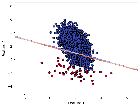
So we see that the recall increases at the cost of lowering the precision. This is confirmed by the decision boundary displacement.
However, here we completely discard the potential effect on the calibration of the model. Instead to check the hard decision boundary, let’s check the decision boundary based on the probability estimates.
fig, axes = plt.subplots(nrows=1, ncols=2, figsize=(12, 5), sharex=True, sharey=True)
for ax, model in zip(axes.ravel(), [logistic_regression, logistic_regression_balanced]):
    disp = DecisionBoundaryDisplay.from_estimator(
        model,
        X_test,
        ax=ax,
        cmap="coolwarm",
        response_method="predict_proba",
        alpha=0.8,
    )
    ax.scatter(*X_train.T, c=y_train, cmap="coolwarm", edgecolors="black")
    ax.set(xlabel="Feature 1", ylabel="Feature 2")
    fig.colorbar(disp.surface_, ax=ax, label="Probability estimate")
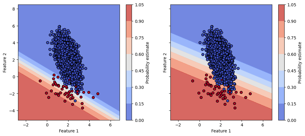
We see that the two models have a very different probability estimates. We should therefore check the calibration of the two models to check if one model is better calibrated than the other.
from sklearn.calibration import CalibrationDisplay

disp = CalibrationDisplay.from_estimator(
    logistic_regression, X_test, y_test, strategy="quantile", name="Unbalanced LR"
)
CalibrationDisplay.from_estimator(
    logistic_regression_balanced,
    X_test,
    y_test,
    strategy="quantile",
    ax=disp.ax_,
    name="Balanced LR",
)
disp.ax_.set(aspect="equal")
_ = disp.ax_.legend(loc="upper left")
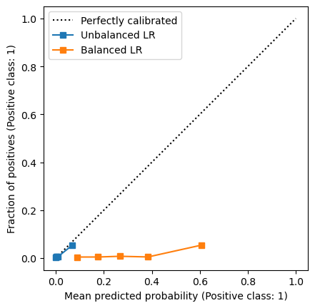
We clearly see that the balanced logistic regression model is completely miscalibrated. In short, this is the effect of resampling. We could have a look at the ROC curves of the two models to check if the predictions ranking changed.
from sklearn.metrics import RocCurveDisplay

fig, ax = plt.subplots()
RocCurveDisplay.from_estimator(
    logistic_regression, X_test, y_test, ax=ax, linestyle="-.", name="Unbalanced LR"
)
RocCurveDisplay.from_estimator(
    logistic_regression_balanced,
    X_test,
    y_test,
    ax=ax,
    linestyle="--",
    name="Balanced LR",
)
/home/runner/work/calibration-cost-sensitive-learning/calibration-cost-sensitive-learning/.pixi/envs/doc/lib/python3.13/site-packages/sklearn/utils/_plotting.py:175: FutureWarning: `**kwargs` is deprecated and will be removed in 1.9. Pass all matplotlib arguments to `curve_kwargs` as a dictionary instead.
  warnings.warn(
<sklearn.metrics._plot.roc_curve.RocCurveDisplay at 0x7fe9f46a6490>
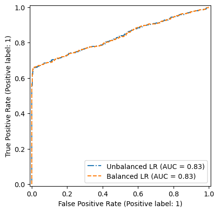
We see that the two models have the same ROC curve. So it means, that the ranking of the predictions is the same.
As a conclusion, we should not use resampling to deal with imbalanced datasets.
Instead, if we are interesting in improving a given metric, we should instead
tune the threshold that is set to 0.5 by default to transform the probability
estimates into hard predictions. It will have the same effect as “moving” the
decision boundary but it will not impact the calibration of the model. We will go
in further details in this topic in the next section. But we can quickly experiment
with the FixedThresholdClassifier from scikit-learn that allows to set a threshold
to transform the probability estimates into hard predictions.
from sklearn.model_selection import FixedThresholdClassifier

threshold = 0.1
logistic_regrssion_with_threshold = FixedThresholdClassifier(
    logistic_regression, threshold=threshold
).fit(X_train, y_train)
fig, axes = plt.subplots(nrows=1, ncols=2, figsize=(12, 5), sharex=True, sharey=True)
for ax, model, title in zip(
    axes.ravel(),
    [logistic_regression, logistic_regrssion_with_threshold],
    ["Threshold 0.5 (default)", f"Threshold {threshold}"],
):
    disp = DecisionBoundaryDisplay.from_estimator(
        model,
        X_test,
        ax=ax,
        cmap="coolwarm",
        response_method="predict",
        plot_method="contour",
    )
    ax.scatter(*X_train.T, c=y_train, cmap="coolwarm", edgecolors="black")
    ax.set(xlabel="Feature 1", ylabel="Feature 2", title=title)
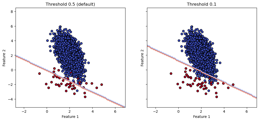
We see that the decision boundary similarly to the balanced logistic regression model. In addition, since we have a parameter to tune, we can easily target a certain score for some targeted metric that is not trivial with resampling.
We can go further and check that the two models that we have are both calibrated the same way.
fig, axes = plt.subplots(nrows=1, ncols=2, figsize=(12, 5), sharex=True, sharey=True)
for ax, model, title in zip(
    axes.ravel(),
    [logistic_regression, logistic_regrssion_with_threshold],
    ["Threshold 0.5 (default)", f"Threshold {threshold}"],
):
    disp = DecisionBoundaryDisplay.from_estimator(
        model,
        X_test,
        ax=ax,
        cmap="coolwarm",
        response_method="predict_proba",
        alpha=0.8,
    )
    DecisionBoundaryDisplay.from_estimator(
        model,
        X_test,
        ax=ax,
        cmap="coolwarm",
        response_method="predict",
        plot_method="contour",
    )
    ax.scatter(*X_train.T, c=y_train, cmap="coolwarm", edgecolors="black")
    ax.set(xlabel="Feature 1", ylabel="Feature 2", title=title)
    fig.colorbar(disp.surface_, ax=ax, label="Probability estimate")
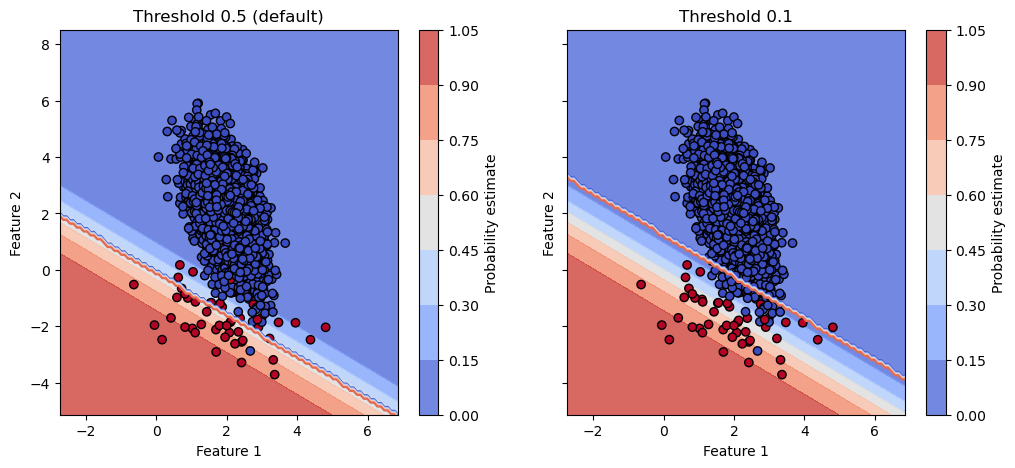
This is not a surprise since the thresholding is a post-processing that threshold the probability estimates. Therefore, it does not impact the calibration of the model.